Plan
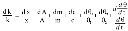
The idea of this experiment is to discover the value of k, the rate of flow of heat through a material per unit area per unit temperature gradient. The units of k are Wm-1K-1 (from Js-1m-1K-1).
What am I going to do?
I have been given a piece of (blue) cloth and I will be using Lees' Disc, described below, to find k. I will be using 'VELA' data logging facilities to collect an accurate and detailed sample of data during the cooling curve.
What is Lees' Disc?
Lees' Disc is an alternative method of finding heat flow, the main other being Searle's bar.
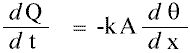
![<-[C]||[B]#[A]->Heat Flow #=Electric Heater Element](Apparatus.gif)
Above is a diagram of the electric version of Lees' Disc. The blue material between discs C and B is the cloth under test. The whole contraption is held together tightly with screws to give good thermal contact.
Why Lees' Disc?
Searle's bar is generally better for (very) good conductors. Lees' Disc is more suited to poor conductors. Cloth is a poor conductor.
In Searle's bar, the x (width of the material) is much greater than A, the area of material in contact with the discs either side, giving a measurable dq/dx. During information gathering conversations with my teachers, I also discovered that Searle's Bar is a very unreliable method if not performed with excellent skill and materials/equipment.
Lees' Disc, on the other hand, gives a measurable dQ/dt.
How will I do it?
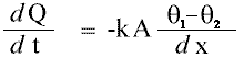
Set up the equipment as shown:
![[C]||[B]#[A] Probes to VELA, heater plugged in.](Setup.gif)
Temperature probes should be calibrated in water first. Between the heater element and the powerpack should be an ammeter (in series) and a voltmeter (in parallel). For good thermal contact between the discs and the probes, put a little oil in the holes.
- Hold the Voltage and Current steady. Heat until the temperatures of B and C stop fluctuating. This means that the heat flowing through the insulator each second is the same as the heat lost by C each second. This assumes that there is no heat loss out of the sides of the sample - this is reasonable since we have a small x and a big A (so very little area out of which to escape).
- When steady, measure the temperatures of A, B, and C (A is not actually needed), the width of the material, as well as the surface area of the material in contact with the disc. Also make a note of the air temperature around the experiment, which should be constant throughout. The temperature of C here is the working temperature.
- Remove the insulator (Warning! Can be hot!). Heat continuously until temperature of X is 5°C greater than it was when you recorded the temperatures.
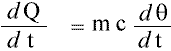
Remove A, the heater, and B. Place a thick strong insulator where the material under test was. Check the VELA probe is still in place.
![[C]|||||| Probe to VELA.](Cooling.gif)
There is now heat loss only in the direction in which heat loss was occuring in the previous section (heating) since the heat loss through the strong insulator is negotiable. When ready (and as quickly as possible), start the VELA program 73 (temperature) with a 2 or 3 second interval. The VELA can only take 512 readings at a time, and the cooling takes around 20 minutes. Take note of the air temperature - it should be the same as in step 3.
- Once finished, measure the mass of the disc, and find it's specific heat capacity (this will be either written on it or available in books).
I will be using brass discs.
Calculation
In step 3, we found A, x, q1, and q2.
In step 5, we found m, c and from the data collected by the VELA we can plot a graph and find the temperature gradient of the cooling graph at the working temperature.
From the above,
dQ/dt is the same each time since the rate of flow through the cloth material is the same as the rate of flow through the brass disc when heating (actually when steady), and the rate of flow when cooling is the same as the heat of flow when steady since it is the same material with the same sides uncovered.
Prediction
In my research I found insulators with k of around 0.01, 0.03 and thereabouts, so it seems reasonable to assume that will be the magnitude of the value of k for this blue cloth.
Results
The raw results are at the back. The data collected by the VELA is on the whole of excellent quality, apart from the first few results (discussed later) there are no unexpected data points.
Graphs
![[Graph 1]](Graph1.gif)
This graph was drawn with a moving average - that is to say, each point on the line is the average of the last 48s's tempertures. No weighting was performed.
![[Graph 2]](Graph2.gif)
This graph was drawn with a moving average too, but this time all the repeated data points were ignored, so the period is not a constant time interval, but simply the last two different data points. This results in a line which is less smooth, but nearer to the data points.
In both cases, the line actually ends up slightly to the right of the data. This is an artifact of the method used. Since each data point is the average of the previous 12 and 2 data points respectively, the temperature for each time will be slightly higher than the actual temperature at that time. This does not affect the gradient since the line is merely moved up, not transformed.
The idea of the averaging is to soften the curve.
Gradient Obtained
When measured by hand, on the first graph, I get a gradient of 2.18×10⁻² ± 1.08×10⁻³*. When done numerically, in the spreadsheet, I get a gradient of 7.64×10⁻³ (note that this value is quoted to 6 decimal places since it is very small and therefore this level of accuracy is waranted). This value is rather different for various reasons, primarily because the computer does not take into account the rest of the curve (when drawing a tangent, even if there is a slight hic-up at the point for which the tangent is needed the human brain takes into account the rest of the curves and extrapolates the gradient). It is still in the same order of magnitude.
*: To calculate the gradients, I used: (note that this is dependant directly on the printed dimensions of my graph, and does not have any relation to Lees' Disc in particular)
((-0.4/1.7)*1+34) / ((0.2/1.4)*200+1600) = 2.07x10⁻² (G1)
((0.6/1.7)*1+34) / ((-0.7/1.4)*200+1600) = 2.29x10⁻² (G2)
(G1-G2) / 2 = the error in the gradient (1.08x10⁻³)
(G1+G2) / 2 = the middle value (most likely to be correct) (2.18x10⁻²)
Data
- A=34.8°C
- B=34.0°C (q1)
- C=29.5°C (q2)
- AIR=20.3°C (this was constant throughout)
- pd=5.1 V (this was constant throughout)
- I=0.29 A (this was constant throughout)
- width of cloth=0.0002m (x)
- contact diameter=0.0040m
- mass=0.1377kg
- specific heat capacity of brass=370 Jkg-1K-1
- gradient of cooling graph at 29.5°C= 2.18×10⁻² ± 1.08×10⁻³
- contact area= 1.26×10⁻⁵m2 (A)
- dq=4.5°C
Value of k obtained
Using the equation given iun the "Calculation" section, and the data in the immediately above "Data" section, k=3.92 Wm-1K-1. I continue getting this, even after intense checking, so either I have made a severe error in some very obscure place or there was some problem in the experiment (see the Limitations section below). I think it is the latter. The reason I think this is a "wrong" value is that it is closer to the value of k for marble (a modest insulator) than for most insulators. Of course, it might be correct! After all, it has been collected emprically, so there must be some measure of truth in it's value.
Errors
The ![]() at the
start of the graph is probably due to the lag between the disc heating
up and the probe heating up. Also, the first few seconds of measuring
still had the heater near the disc (I was still setting up the
apparatus for cooling). This has no particularily bad effect on the
experiment and so can be ignored safely.
at the
start of the graph is probably due to the lag between the disc heating
up and the probe heating up. Also, the first few seconds of measuring
still had the heater near the disc (I was still setting up the
apparatus for cooling). This has no particularily bad effect on the
experiment and so can be ignored safely.
The actual error can be calculated by:
Which can be simplifed quite a lot. To start with, the dc/c is laughibly small (since it is the "official" value) and can be removed completely. Secondly, that odd looking construction at the end (which represents the error in the gradient) can be turned into (G1-G2) / (G1+G2) where G1 and G2 are the low and high gradients respectively. Finally, dm/m is also very small (around 0.0005g error) and can be dropped. This leaves:
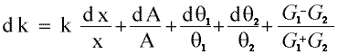
- dx=quite big,I would say ± at least 1mm (0.0001m) - see the limitations section.
- dA=error in diameter squared, that is 1.6×10⁻⁹ (0.0004m is the accuracy of the human eye, unaided)
- dq=The VELA was very accurate (2 of the probes were out of synch with the others other, but there was a constant difference and in any case they were used for the Air and A disc so they were never actually used numerically); according to VELA documentation, 0.05ºC
- Gx=The error values for the gradient are discussed in the "Gradient" section.
I therefore make the absolute error to be 2.17 (about 55%) !!! This is largely due to the error in width (0.5, the others only come up to the 0.05). This also means that the value of k obtained could mean anything from 1.75 to 6.09 Wm-1K-1.
Limitations and Evaluation
The most important limitation/problem is the width of the cloth. When I placed the cloth in, I tightened up the bolt a lot. This means that the air was all squeezed out, so the cloth was probably no longer the insulator I expected. This is not such a bad problem really, since if we were looking for Air's k we would do that seperately. It is quite likely that the cloth was really only 0.5mm wide during the experiment, even smaller than I have suggested in the "Errors" section above.
Another problem I had was that I had to do the experiment twice - the first time, when I did the decay graph I opted for two seconds as planned but it finished it's 512 readings at 29.7°C, making the graph useless since one needs the working temperature to be in the middle. So I redid the entire experiment (I had to do the first bit too because this was 2 days later and the room temperature had changed), and used a four seconds interval instead. In hindsight, it is obvious that quite unlike my estimated 20 minutes, it takes around 25 minutes to cool the disc.