The Physics of Ultrasound
The Physics of Waves
There are two types of waves: longitudinal waves and transverse waves. Longitudinal waves are waves in which the direction of particle motion is parallel to the direction of the wave energy propagation, and transverse waves are waves in which the direction of particle motion is perpendicular to the direction of the wave energy propagation.
Sound waves are mechanical pressure waves. Like all such waves, they must have a medium in which to propagate — typically this is air, but other materials such as water, brick and human tissue are equally able to support sounds waves. Pressure waves are always longitudinal waves (see figure 1).
The frequency (f) of a pressure wave is defined as the number of high/low pressure regions crossing a point per unit time (units s-1 or Hertz, symbol Hz). The wavelength (λ) of a pressure wave is measured from one rarefaction to the next rarefaction. The speed (c) (or wave velocity) of pressure waves travelling through a propagation medium is defined by the equation:
| c = λ f |
![]()
▲ Figure 1: Longitudinal Waves.
...and is the length of wave that crosses a point per unit time (units ms-1). The amplitude (ΔP) of a wave is the difference between the pressure at rarefaction (or compression) and the ambient pressure. The impedance (z) of the propagation medium is vital in order to predict the magnitude of the reflected echoes at interfaces between two different tissues. The impedance of a medium is defined by following relationship:
| z = ρ c |
...where ρ is the density of the medium.
The physics of ultrasound waves differs from that of waves in the audible range in ways, for example molecular relaxation effects become more apparent at higher frequencies.
The Physics of Ultrasound
The range of human hearing is generally accepted to be 20 Hz to 20 kHz; ultrasound waves are those sound waves whose frequencies are above this range. They generally obey the same rules as all sound waves.
The Wave Equation for Ultrasound
The 1D wave equation for sound waves is as follows:
|
∂2 ΔP
∂t2 |
- | c2 |
∂2 ΔP
∂x2 |
= | 0 |
However, sound waves only travel in only one dimension in very specific cases (for example, in infinitely narrow pipes). In general, sound waves travel in three dimensions. The 3D wave equation for sound waves is as follows:
|
∂2 ΔP
∂t2 |
- | c2 | ( |
∂2 ΔP
∂x2 |
+ |
∂2 ΔP
∂y2 |
+ |
∂2 ΔP
∂z2 |
) | = | 0 |
In both these equations, the speed of the wave, c, is given by the following expression:
| c | = | √( |
B
ρ |
) |
...where B is the bulk modulus of the fluid (and is a function of ΔP, which, of course, is itself a function of x, y, z and t).
Ultrasound Imaging
Basic Premise
▼ Wave velocities for parts of the human body.
| Medium | c / ms-1 |
|---|---|
| Air | 330 |
| Water | 1480 |
| Fat | 1450 |
| Blood | 1570 |
| Kidney | 1560 |
| Soft tissue (average) | 1540 |
| Liver | 1550 |
| Muscle | 1580 |
| Bone | 4080 |
The relatively slow wave velocity in tissues enables distance measurements to be made. The amount of time it takes for a sound wave to travel from a transducer (transmitter/receiver unit) to a reflector (e.g., a tissue boundary) and back can be measured, and, along with the known wave velocity, can then be used to calculate the separation distance.
Ultrasound echoes are produced by two kinds of reflectors: specular and diffuse.
High Amplitude Echos: Specular Reflectors
Specular reflectors are large interfaces in the body between two different soft tissues, such as the edge of a liver or kidney. If a sound ray is incident on such an interface, two rays are produced: a transmitted ray, which propagates into the second soft tissue, and a reflected ray, which propagates back into the first soft tissue. The greater the difference in impedance (z1-z2) of the two materials, the greater the bias towards reflection.
This is obvious from the equation defining the reflection coefficient (R):
The reflection coefficient gives the ratio of the amplitudes of the reflected wave to the transmitted wave. Hence if R=1, then the wave is completely reflected.
| R = |
z1 -
z2
z1 + z2 |
The direction of the reflected ray (the echo) is governed by the laws of reflection, which state that the angle of incidence equals the angle of reflection. For single transducer pulse-echo equipment to register the reflected echo, it must be backscattered at an angle of π radians and back to the front face of the transducer. So only when the incident beam is perpendicular to the interface will the reflected beam be received by the transducer (i.e., only when the angles of incidence and reflection are both 0).
Low Amplitude Echos: Diffuse Reflectors
Diffuse reflectors have physical dimensions that are much smaller than the acoustic wavelength. Point reflectors and interface roughness are common examples of diffuse reflectors. Diffuse reflectors scatter ultrasound in all directions, thus producing low-amplitude echoes. Slight local variations in acoustic impedance inside body organs also act as diffuse reflectors.
Generating and Detecting Ultrasound
Ultrasound is produced using devices called transducers. These devices use piezoelectric crystals, in which a varying voltage causes a correspondingly varying strain. By varying the input voltage at a suitably high rate, ultrasound waves are produced.
Transducers have a range of frequencies which they are able to produce. This is known as the bandwidth.
Similarly, by varying the strain on the piezoelectric crystal, a correspondingly varying voltage is produced.
Since these processes are reversible, the same device can be used to both transmit and detect the waves. This greatly simplifies the design.
The Pulse-Echo Principle
Ultrasound is not emitted continuously from the transducer, as that would make echo-detection useless (there would be no way of knowing how long a wave had been travelling once it returned to the transducer). Instead, transducers oscillate between two modes. First a pulse of ultrasound is emitted, and then in the pause that follows the time that elapses for the echos to be detected is measured.
The distance can then be calculated using the following equation:
| r = ½ c Δt |
The intensity of the echos is also recorded, and is used when rendering the scans.
Figure 2 (below) shows the transducer is shown transmitting into the patient. The circles indicate operator controls that affect the echo amplitude data written into the ultrasonic image. Note also the echo waveforms at various stages of signal processing, shown at the top of the figure.
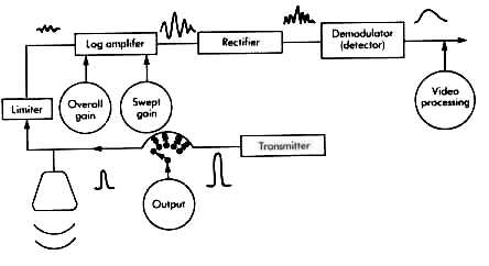
The Limiter
Its function is to protect the rest of the receiver from the high-transmitter voltages. Because both the transmitter and the receiver are connected to the transducer, the transmitter is connected directly into the receiver. If the high-transmission voltages were to enter the receiver unattenuated, it would saturate the receiver for a relatively long period of time, obscuring any shallow echoes. The limiter is a circuit that passes low-amplitude signals (echoes) unaffected but in order to protect the receiver, it limits or clips any high-amplitude signal that is above a predetermined threshold.
The transmitter circuit produces a high-amplitude, short duration pulse. The output control then attenuates the amplitude of the shock pulse, before applying it to the transducer.
After each transmission pulse the transducer then receives its returning echoes. After the received echoes are converted into weak voltage waveforms by the transducer, they are processed by the receiver. The receiver is actually made up of many smaller sub-circuits, each one performing a specific signal processing function. The first sub-circuit is the limiter (see sidebar). The second is the log amplifier. The log amplifier amplifies the weak echo signals by over 100 dB.
Next, the echo signals enter the rectifier sub-circuit, where the negative half-cycles in the echo voltage waveforms are converted into positive half-cycles. Then, with demodulation, the fundamental frequency signal on which the echo amplitude information has been carried is eliminated, leaving only the so-called envelope (i.e., magnitude) of the echo signal.
The output of the demodulator is the amplitude of the echo signal and its time delay from the transmission pulse. Homogeneous soft tissues in the body should appear uniform in the ultrasonic image. However, echo amplitudes received from deeper soft tissue structures have lower amplitudes because of the attenuation of the overlying tissue. This leads to a graded appearance of the tissue gray-scale image.
This problem is solved by a method called time gain compensation. This is a method of time-increasing the gain of the log amplifier, in sync with the arrival of lower and lower amplitude echoes from deeper and deeper in the body. The voltage that controls the gain of the log amplifier is usually varied linearly with an operator selectable slope. Thus, by proper selection of the operator selectable slope of the swept gain, the effects of tissue attenuation in the image may be compensated.
Output
Cathode Ray Tubes (i.e., TV or computer screens) are used as the display in most ultrasonic imaging systems. The screen acts as a two-dimensional surface to display the echo data in a two-dimensional format, plotting the amplitudes as variations in brightness.
A-Mode Display
An A-Mode scan the data for only a single line-of-sight from the transducer. The horizontal axis represents the time after the pulse and the vertical axis the amplitude of the amplified and demodulated echoes measured at that time.
Note the large first pulse, called the "main bang". It is produced by the reception of a clipped transmission pulse, and indicates the spatial position of the transducer front face.
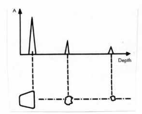
▲ Figure 3: A-Mode.
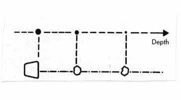
▼ Figure 4: B-Mode.
The horizontal axis is calibrated in distance, which means that the equipment, even though it is always making time measurements of the returning echoes, is converting the measured times into depths in the patient. Thus the plot can also be interpreted as depth against boundary. A peak represents a sharp boundary (e.g., bone to water), a steady low line represents a homogenous section (e.g., inside a muscle).
B-Mode Display
A B-Mode (brightness mode) display plots the same data as an A-Mode display, but with brightness representing echo amplitudes instead of a vertical trace. A set of B-Mode image lines scanned through a cross section of the patient (also called a scan plane) generates a gray scale image in which the echo amplitudes are encoded in image shades of gray. Gray scale displays present both specular and diffuse echoes for diagnosis.
Attenuation
Definition
Attenuation is loss of strength of a signal. In the case of ultrasound imaging, attenuation refers to the reduction in signal strength as the waves travel through the patient.
After being emitted from the transducer, the sound energy travels into tissue confined along a pathway known as the beam pattern. In a non-scattering and non-absorbing medium, the energy in the ultrasound pulse remains constant. However, as the beam pattern becomes wider, the acoustic intensity decreases (since the energy must be disturbed over a larger area). This change of intensity as the beam widens causes depth variations in the amplitudes of the received echoes from identical reflectors.
As the ultrasound wave moves through the tissue, the tissue particles are set into motion. In a non-absorbing medium, as the waves passes by, the particles give back their vibrational energy and the wave-particle combination conserves energy. In tissue, however, the particles lose some of their vibration energy to frictional effects or to other internal modes of tissue motion and energy is absorbed as tissue heat energy. This causes the overall intensity of the signal to decrease.
Whenever there is a difference in acoustic velocity across an interface, the direction of the transmitted ray is shifted slightly as it crosses the interface. This phenomenon is known as refraction. As in optics, the magnitude of the directional change may be calculated from Snell's law.
Doppler Effect
In terms of medical ultrasound, the Doppler effect is a change in frequency of the received echoes (compared to the frequencies of the transmission pulse), due to the target moving relative to the front face of the transducer. In a pulse-echo ultrasonic measurement with the source and receiver being the same, the reflector motion causes a frequency difference between the received and transmitted frequencies to be as in the following equation:
| Δf | = |
2 v F0 cos θ
c |
The Doppler shift is greater when the reflector is moving either directly toward or away from the transducer. When the reflector is moving toward the transducer the Doppler shift is positive (the received frequency is greater than the transmitted frequency). When the reflector is moving away from the transducer, the Doppler shift is negative (the received frequency is lower than the transmitted frequency). When the reflector is moving in a direction perpendicular to the beam axis, there is obviously no Doppler shift of the received echoes.
...where: Δf is the Doppler shift frequency, v is the reflector's velocity, F0 is the transmitted frequency, θ is the angle between the beam axis and the reflector, and c is the wave velocity.
The Doppler effect allows the examination of human blood flow without the need to inject radioactive compounds or other dyes into the circulation, nor the need to use X-rays. Although in recent years the clinical use of Doppler ultrasound instruments has become widespread, its role has been confined to answering qualitative questions about flow in relatively large vessels. This method is not yet a quantitative technique capable of measuring such important haemodynamic variables in the body as flowrate, pressure and resistance in large vessels and showing the presence or absence of flow in tissue itself, although work is progressing in this area. Laboratory investigations include the analysis of the interaction of ultrasound with moving blood as well as the dynamic characteristics of blood flow and the vessels themselves.
Other Medical Uses of Ultrasound
Ultrasound is not only used for imaging, however. Here are a few other uses of ultrasound in medical settings:
Safety
Ultrasound is a technique, unlike x-rays, where one does not get exposed to any kind of radiation. The key is to limit the acoustic output of ultrasonic devices to levels which are known not to be hazardous. Knowledge of two indices have been observed to provide feedback to users on potential hazards: the thermal index, which specifies the ability of raising the temperature of tissues, and the mechanical index, which observes the potential for the ultrasonic field to generate acoustic cavitation (making bubbles in fluids). So far, no major harmful effects linked to ultrasound in cells of animals and humans have been demonstrated.
Kidney stone disintegration is rendered possible by the fact that small particles can break when subject to resonant or critical frequencies.
Dental plaque is removed by a narrow high-speed stream of water under the impetus of (generally) 25 kHz signal introduced into the stream.
Since the molecular relaxation processes result in heat generation in a solid, liquid or semi-liquid medium, ultrasound can be applied to affected areas to ease muscular soreness.
Ultrasonic cleaners are used to clean operating tools and other utensils. The acoustic energy is generally transmitted into a detergent fluid in which the utensils are submerged.
Current research at the New York University Medical Center indicates a great deal of promise in the use of ultrasound to treat skin cancer.
Clinical studies are being conducted in the use of ultrasound to unclog blood vessels affected by arteriosclerosis.
Conclusion
The ability to "see" inside somebody's body without causing any harm to the body is extremely useful. However, this technique is only just beginning to be exploited. For example, ultrasound imaging has only been used on pregnant women for the past 35 years. As research into the subject continues, the use of ultrasound in medicine is bound to increase.
Bibliography
J. Zagzebski (1996). Essentials of Ultrasound Physics. London: Mosby.
W. Hedrick, D. Hykes, D. Starchman (1992). Ultrasound physics and instrumentation. London: Mosby.
G. Raina (1997). Obstetric Ultrasound. http://www.wwonline.com/~nvaswani/gunjan/main.htm
V. Humphrey (1998). Medical Ultrasound. http://www.bath.ac.uk/~pysvfh/med_ultra.html
P. Burns (1999). Medical Biophysics. http://pmate01.oci.utoronto.ca/faculty/burns/medbio.burns.html